I chose to do the NeRF project for my final project, which aims to train neural networks to generate 3D objects from 2D images through an interpolation approach between the scenes.
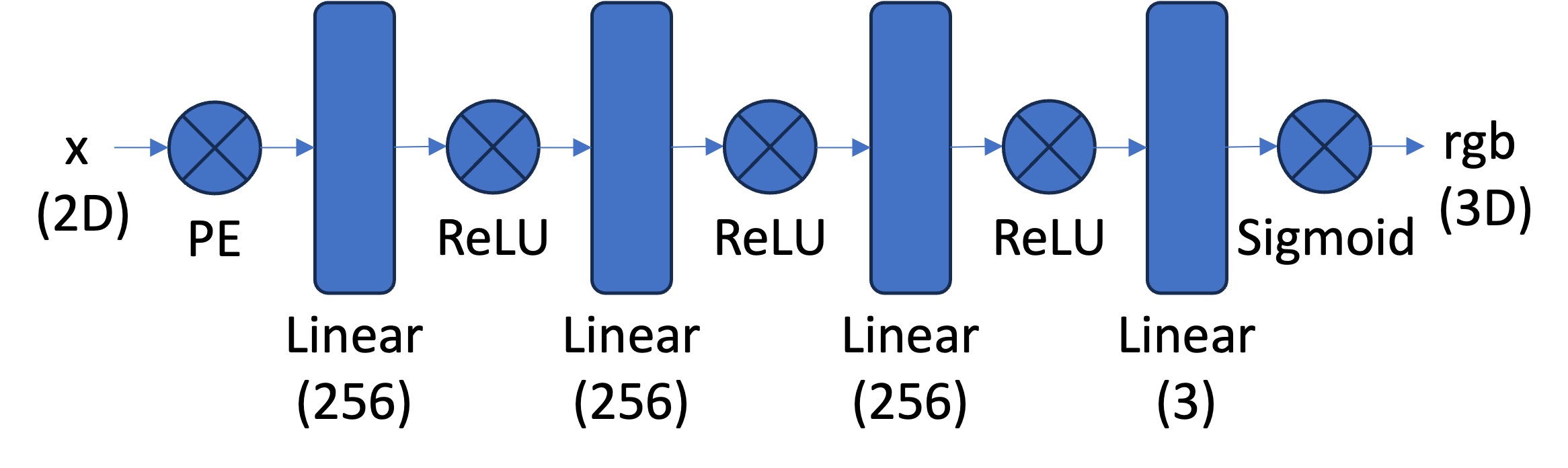
We first start with a neural field that fits and represents a 2D image. The Multilayer Perception (MLP) network usese Sinusoidal Positional Encoding (PE) that maps the u, v coordinates of the image to rgb in 2D. The architecture is shown below - given a 2D input $x$, we first compute the PE, then have 3 linear layers with hidden dimension 256 followed by ReLU, then one final linear layer with hidden dimension 256, and finally a sigmoid at the end to give us the rgb output in 3D.
Now, we do a hyperparameter sweep on the hyperparameters L, which is the highest frequency level in PE, and the learning rate of the MLP.
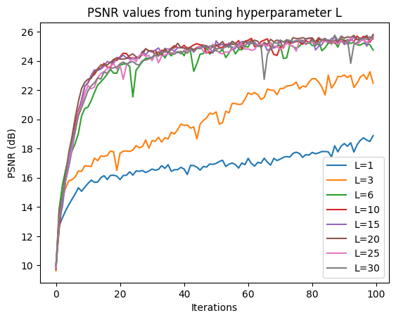
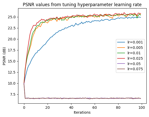
Observing these two graphs, $L = 10$ and $\text{learning_rate} = 0.025$ achieve the highest PSNRs. Now, we can use these values, along with hidden dimension 256 and batch size 10,000 (as described in the spec and architecture), to train the model and generate reconstructed images throughout training.
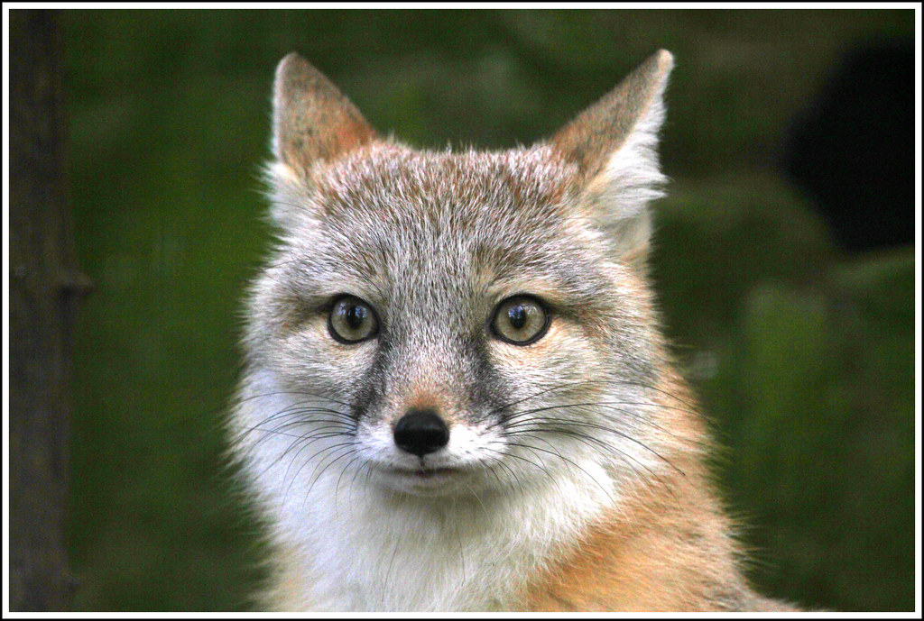
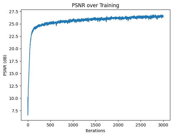
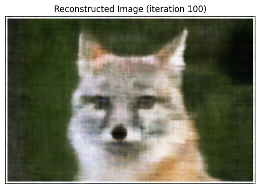
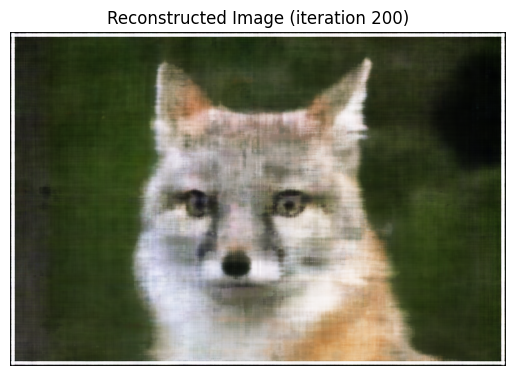
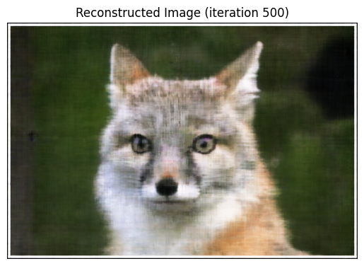
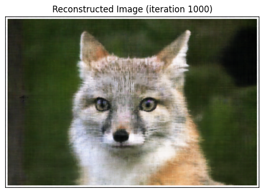
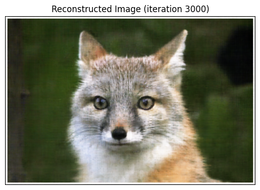
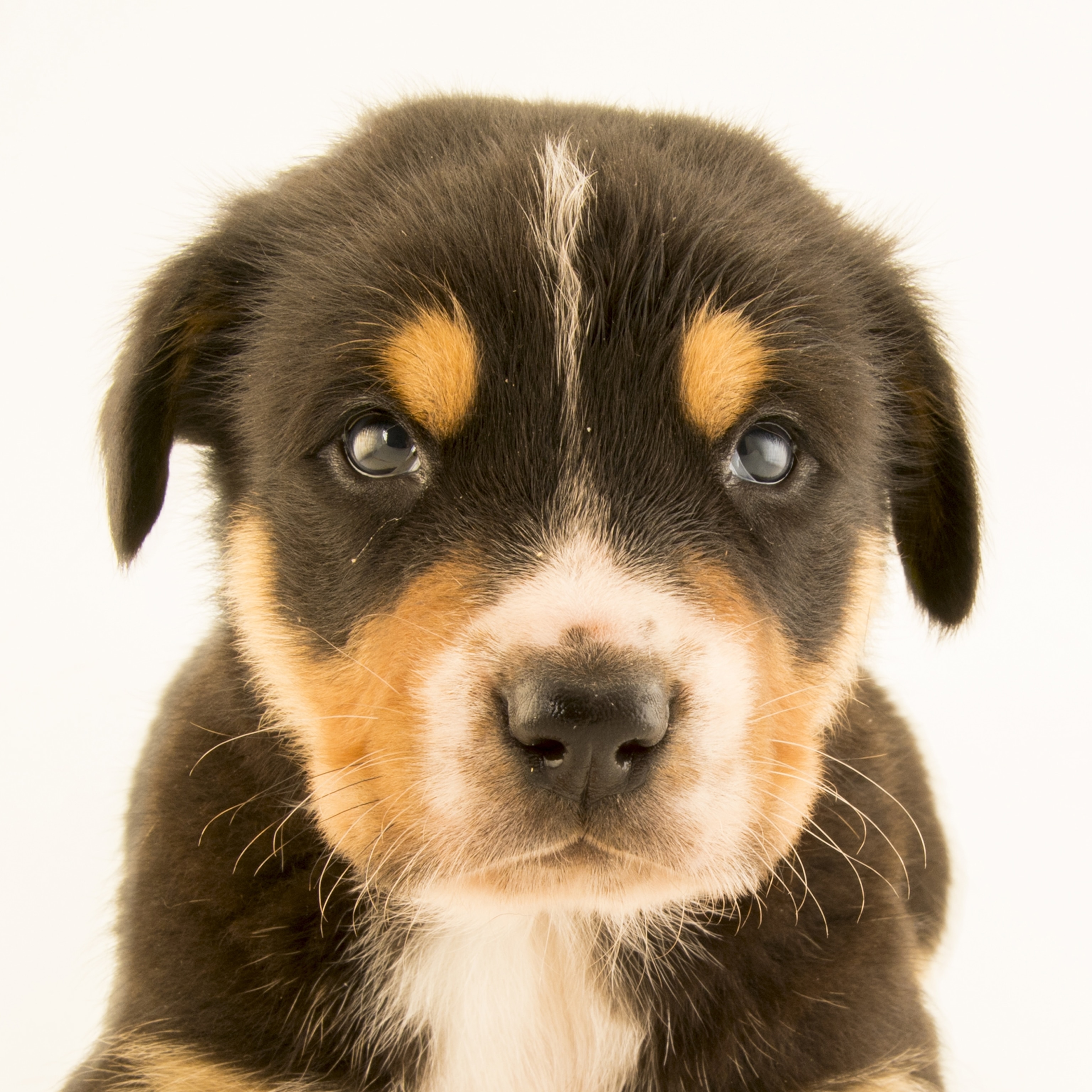
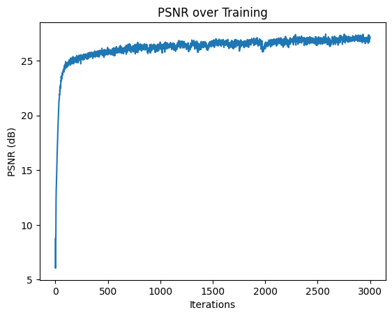
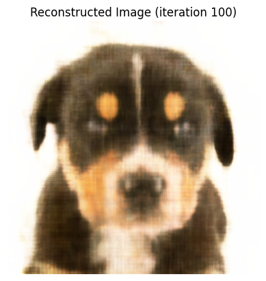
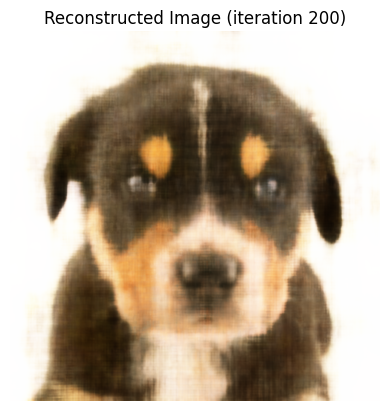

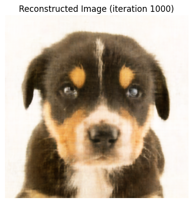
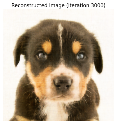
The training took much longer for my dog image than the fox one because the dog is 3072 x 3072 while the fox is only 689 x 1024. We can see the our neural network learns quite quickly how to reconstruct the image as it initially is able to get most of the details, except from some blur, but within a few hundred iterations, the reconstructed image very closely resembles the original one.
Now, we can use a neural raidance field to represent images in the 3D space. We will use the Lego scene (200 x 200 images) from the original NeRF paper.
To convert camera to world coordinates, we use the following equation, where subscript $w$ coordinates are in the world space, subscript $c$ coordinates are in the camera space, $\mathbf R_{3x3}$ is our rotation matrix, and $\mathbf t$ is our translation vector:
To convert pixel to camera coordinates, we use this intrinsic matrix $\mathbf K$, where $f_x$ and $f_y$ is our focal length and $\sigma_x$ and $\sigma_y$ (the midpoints of the image width and height, respectively)$ is our principal point.
To convert pixel to ray (and get the ray origins and directions), we use the following formulas
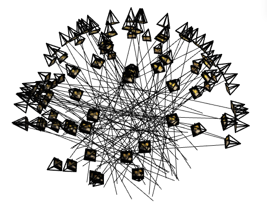
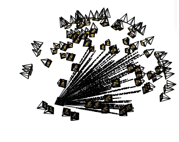
To sample rays, we can first discretize them into samples in 3D space by uniformly creating them along the rays. In the process, we introduce small perturbations only during training so that we touch every point along the ray.
With this, we can create a viser server and get the following two images to
verify we have implemented everything so far correctly.
Now, we can train our model, using volume rendering volrend - adding contribution
of small intervals to the final color like shown in the formula below, where $\mathbf c_i$ is
color at location $i$ we get from our model, $T_i$ is the probability of the ray not
terminating before $i$, and $1-e^{-sigma_i\delta_i}$ is the probability of terminating at $i$.
Our architecture is as follows.
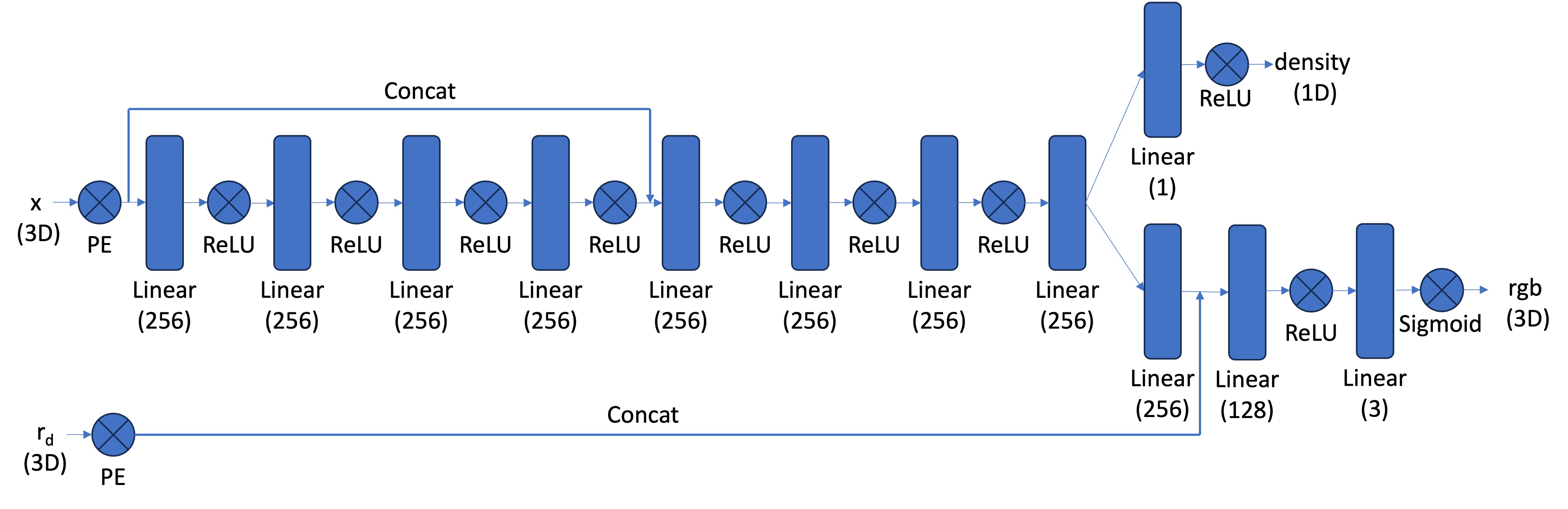
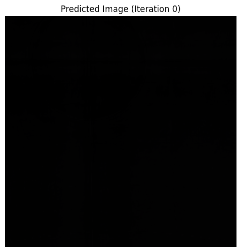
During the training our model, we can visualize the model's predicted image on one of the validation camera views.
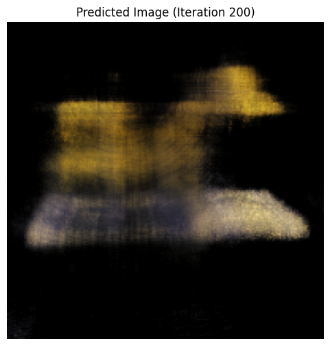
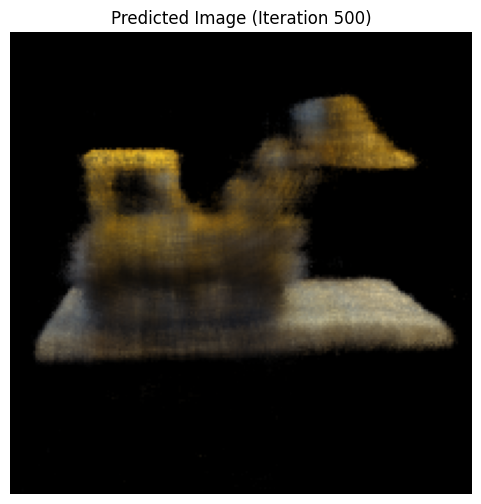
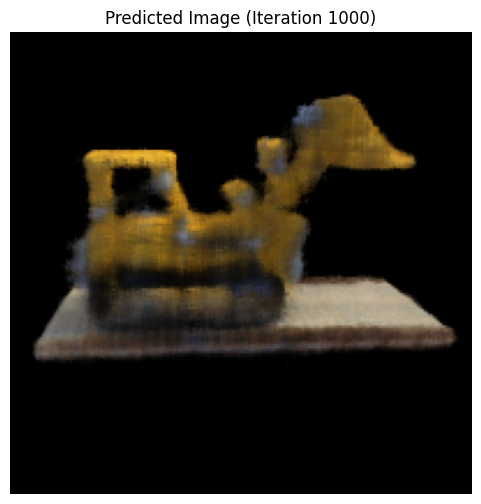
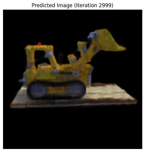
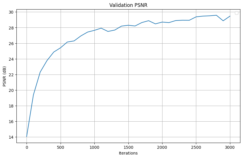
Here is the PSNR of our model throughout training. We can see that it reaches 23 PSNR around 300 iterations and somewhat converges. The training after 1k iterations introduces slightly finer structure, like making the lines and space between its protruding arms clearer.
Finally, we can make a GIF by transforming each of the images/cameras with our trained model.
For the Bells and Whistles, I chose to do "Render the Lego video with a different background color than black..."
To achieve this, we can modify the volrend function to take in a background color
of a tensor with three values for RGB. Previously, volrend didn't explicitly add
additional background color contribution after getting the colors from our density and RGBs so
it's the same as setting the background color to black, which is rgb 0, 0, 0. We will add this
code to the end: compute the remaining transmittance and add the color contribution to the
original color we previously got from the original volrend.
This are two resulting GIFs with a background color of white and purple.